This is a new article series where we will use UNITRONICS’ UniStream® series and UniLogic to perform various verifications. In the 4th episode, we will explain the use and wiring of Local IO.
- UNITRONICS US5-C10-TA30
Now, let’s enjoy FA!

Reference Link
Implementation Wiring
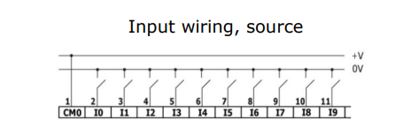
Below is a wiring example for the digital input (source) of the US5-C10-TA30.
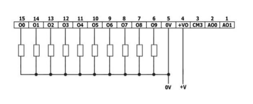
Below is a wiring example for the digital output of the US5-C10-TA30.
Below is a wiring example for the analog input of the US5-C10-TA30.
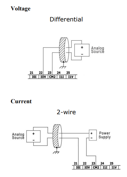
The US5-C10-TA30 has two analog inputs; for analog input 0, wire to I0I for current input and to I0V for voltage input. For analog input 1, please use I1I and I1V.
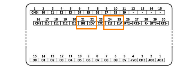
This video allows you to check the terminal block of the US5-C10-TA30.
Implementation IO Tags Setup
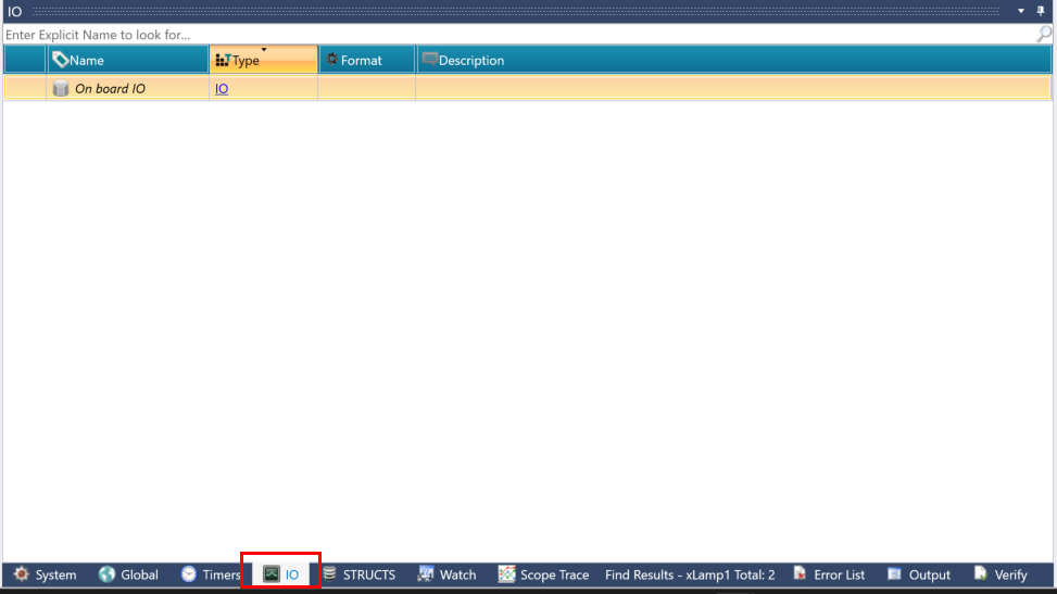
Next, I will introduce how to access the IO on the device itself from UniLogic and the Tags. Open the IO Tab in UniLogic.
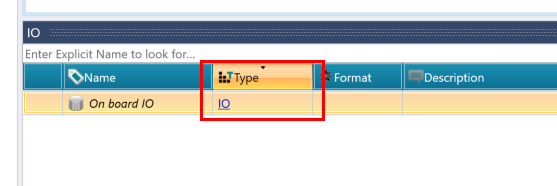
In UniLogic, variables of the IO Type are already declared by default; please click on that IO data type.
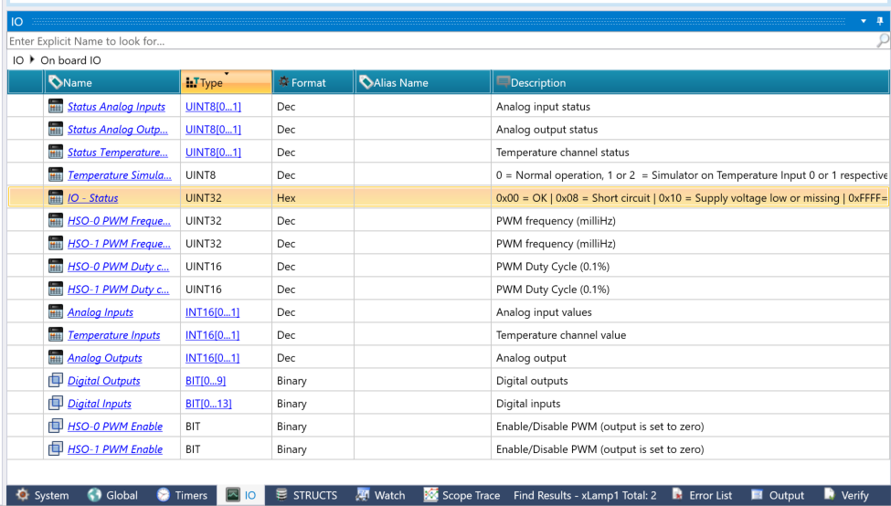
Various variables for obtaining IO status are already prepared in UniLogic.
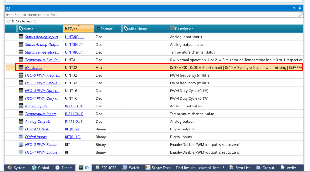
For example, in the IO-Status below, you can check states such as whether the device’s local IO is short-circuited.
Implementation IO Setup
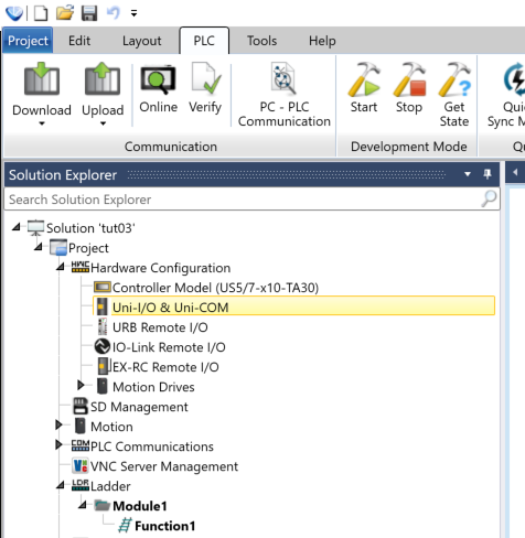
Next, perform the local IO setup for the US5/7-x10-TA30 on UniLogic. Click Project → Hardware Configuration → Uni-I/O & Uni-COM.
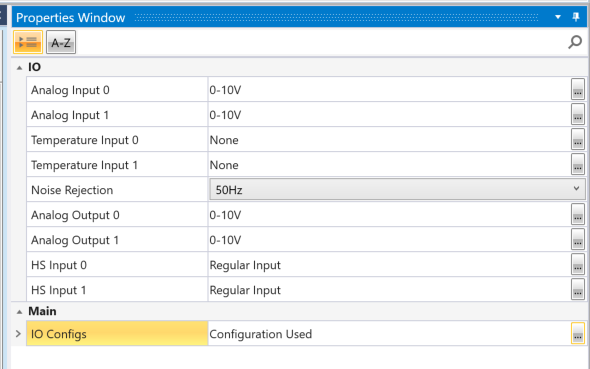
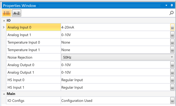
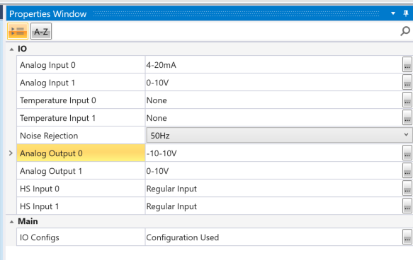
In the Properties Window, you can change the settings for analog inputs/outputs and temperature inputs.
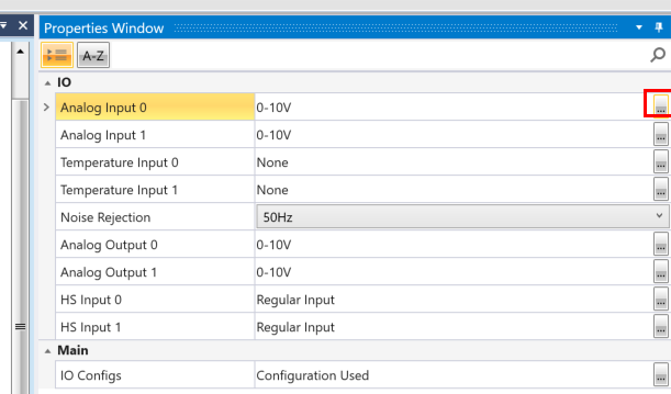
For example, if you want to change the input type of analog input 0 shown below, click the … button.
The analog input settings screen will be displayed.
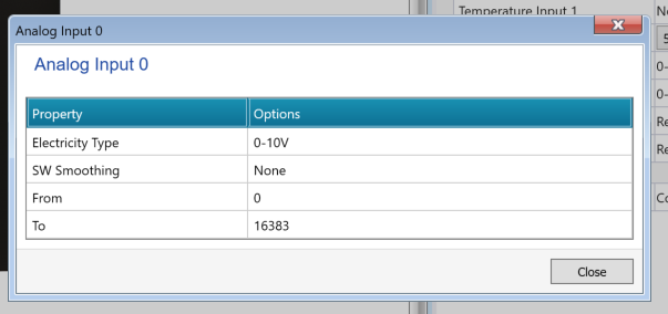
Here you can set the analog input to voltage or current type, range, etc.
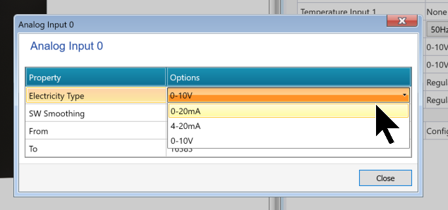
Done! Now analog input 0 is set to 4-20mA.
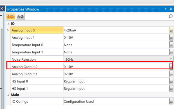
The same operation can be used to change settings for analog output.
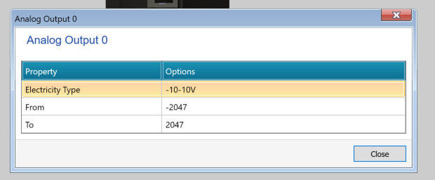
This is the analog output settings screen.
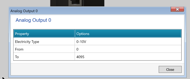
The analog output was set to convert from -10 to 10V into -2047 to 2047.
Done!
Implementation Screen Comments
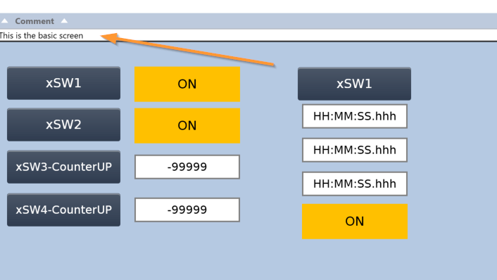
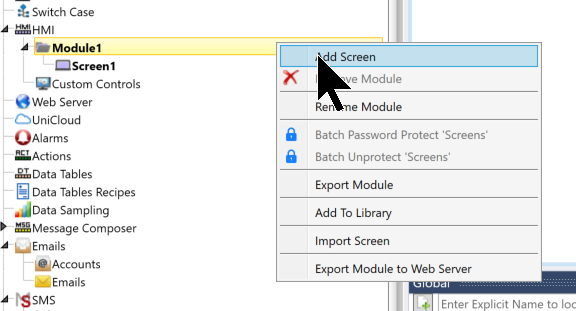
When designing screens on UniLogic, you can add individual comments to each screen.
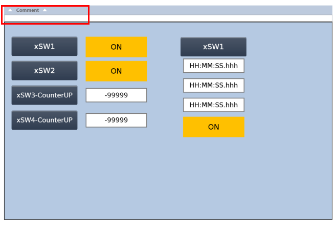
Let’s add a comment from the place indicated by the arrow in the figure below.
Implementation Region
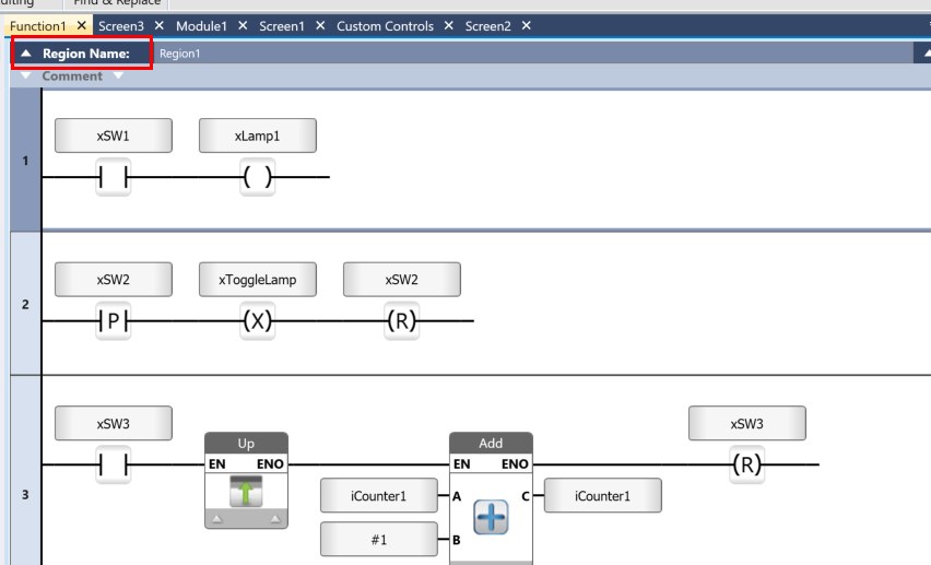
Next, assign a “Region name” to each ladder Function. Open the ladder program and use the “Region” at the top left to divide areas according to the program content, building a more readable program.
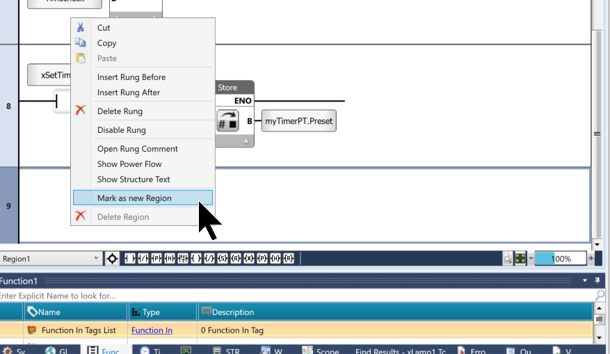
It is also possible to add a new Region within the ladder program by right-clicking on an empty part of the ladder and clicking “Mark as new Region”.
Done! Now a new Region is created.
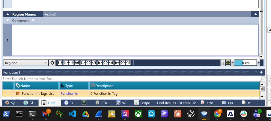
Dividing Regions according to the program’s purpose can improve program readability.
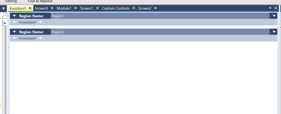
Individual comments can also be entered for each Region.
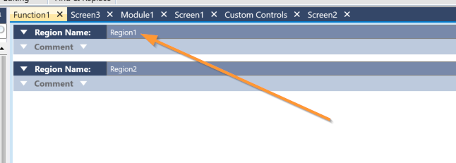
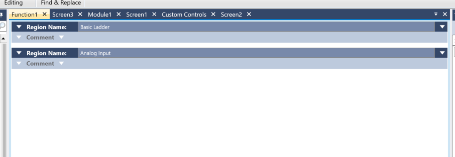
Done! As shown in the figure below, Region 1 is Basic Ladder and Region 2 is Analog Input.
Implementation Linearization Program
Next, scale the analog input data. Add the Math → Linearize function.
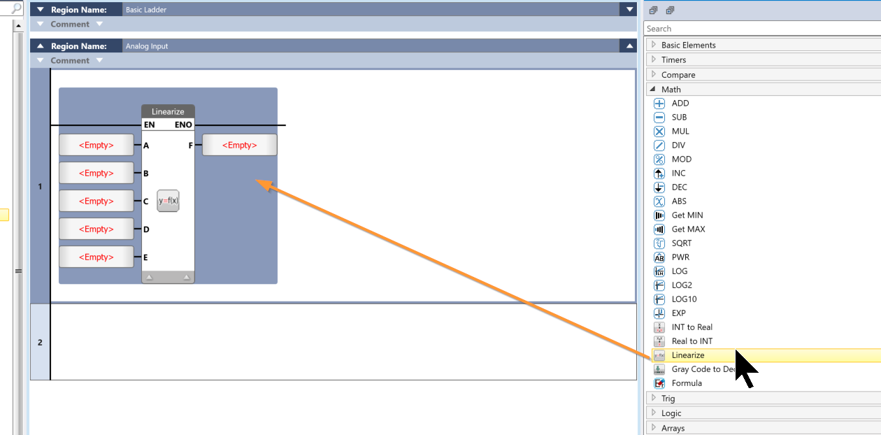
Next, select the Analog Inputs variable from the IO Tab.
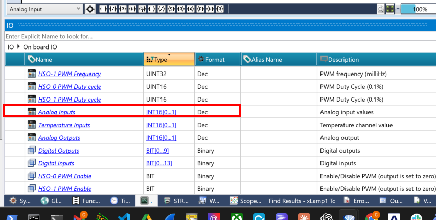
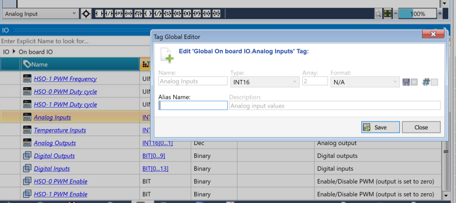
Enter the variable name in the Alias Name column.
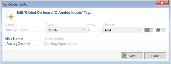
In this article, the analog input variable name will be iAnalogChannel.
Done!
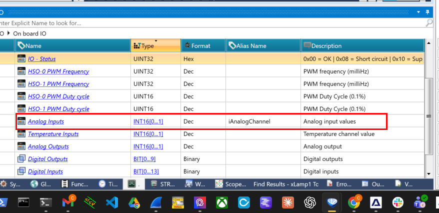
This allows the program to use the analog input variables.
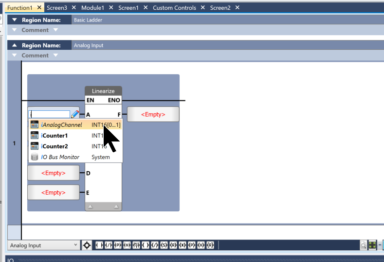
For example, if you want to use analog input Channel 0, set it to iAnalogChannel → Analog Inputs_0.
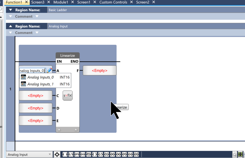
Linearize Function Block
Linearization is a feature for converting values. For example, it can convert an analog input value into a Celsius temperature value.
Operation Example
When X1=0, Y1=0, X2=1023, Y2=1000, the output value is linearized as shown in the graph.
- An analog input of 5.0V is converted to a digital value of 500.
- An analog input of 10.0V is converted to a digital value of 1000.
Parameter List
Symbol | Parameter Name | Description |
|---|---|---|
A | Input Value | Input value for linearization. Single registers, arrays, or structures can be specified. |
B | X1 Value | First known input value in linearization. |
C | Y1 Value | Output value corresponding to the X1 input value. |
D | X2 Value | Second known input value in linearization. |
E | Y2 Value | Output value corresponding to the X2 input value. |
F | Resulting Value | Output value after applying the linearization formula. |
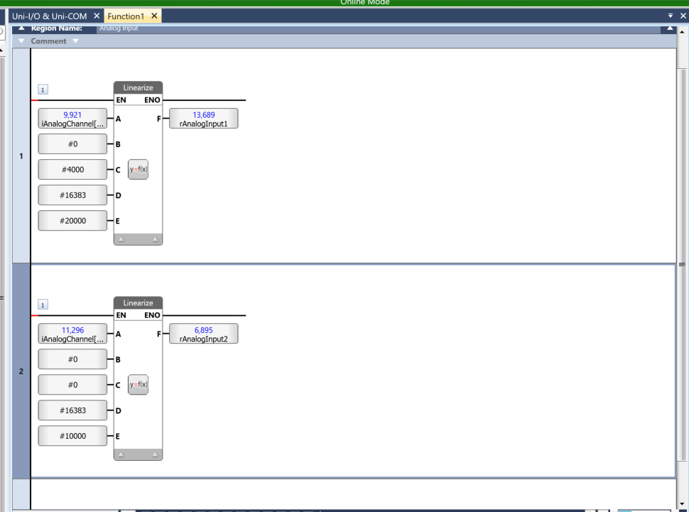
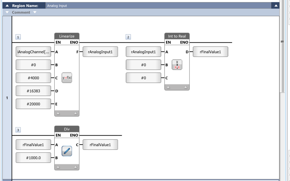
Next, simply link parameters A/B/C/D/E to the appropriate variables from the program.
Results
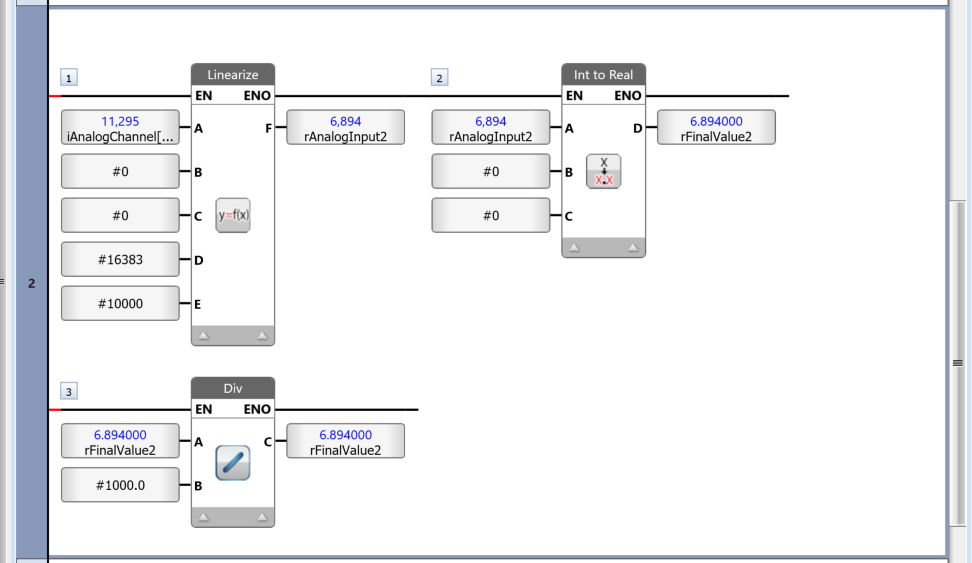
As shown in the figure below, analog inputs Channel 0 and Channel 1 have also been scaled.
Integer to Real Conversion
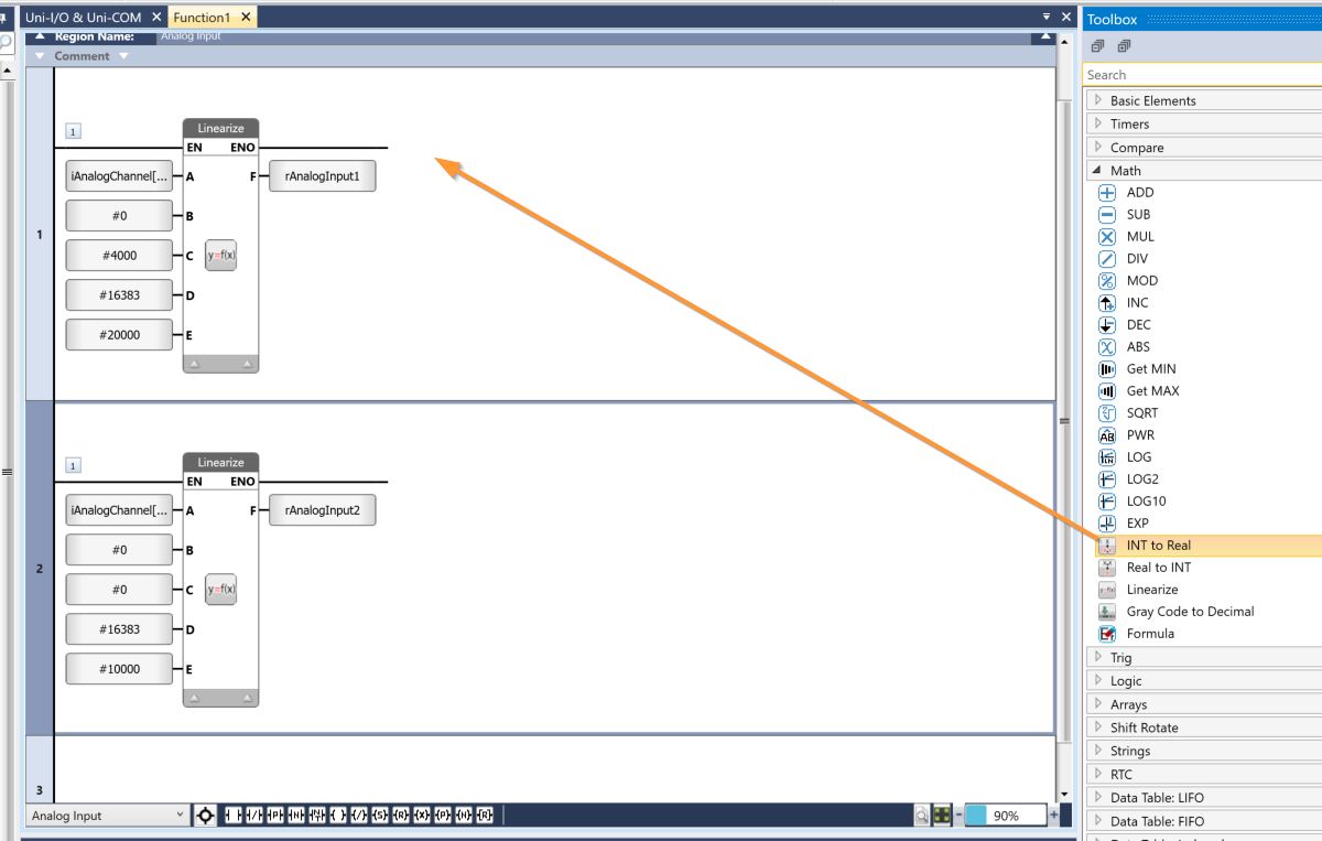
Since the output of the Linearize function is an integer, use the INT to Real function to convert the result into a real-type variable.
Done!
Results
As shown in the figure below, rFinalValue2 became 6.894000 thanks to the Int to Real function.
Implementation – Screen Verification
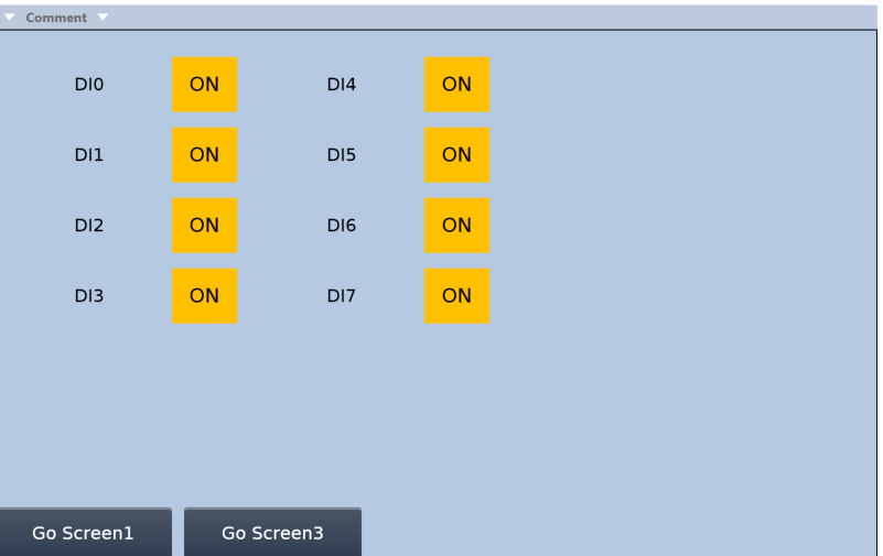
First, create a screen to check the Local digital inputs.
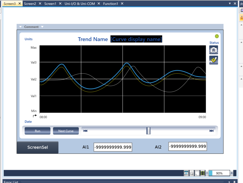
Next, add Graphs/Meters → Cyclic Live Trend to view the variables through tracing.
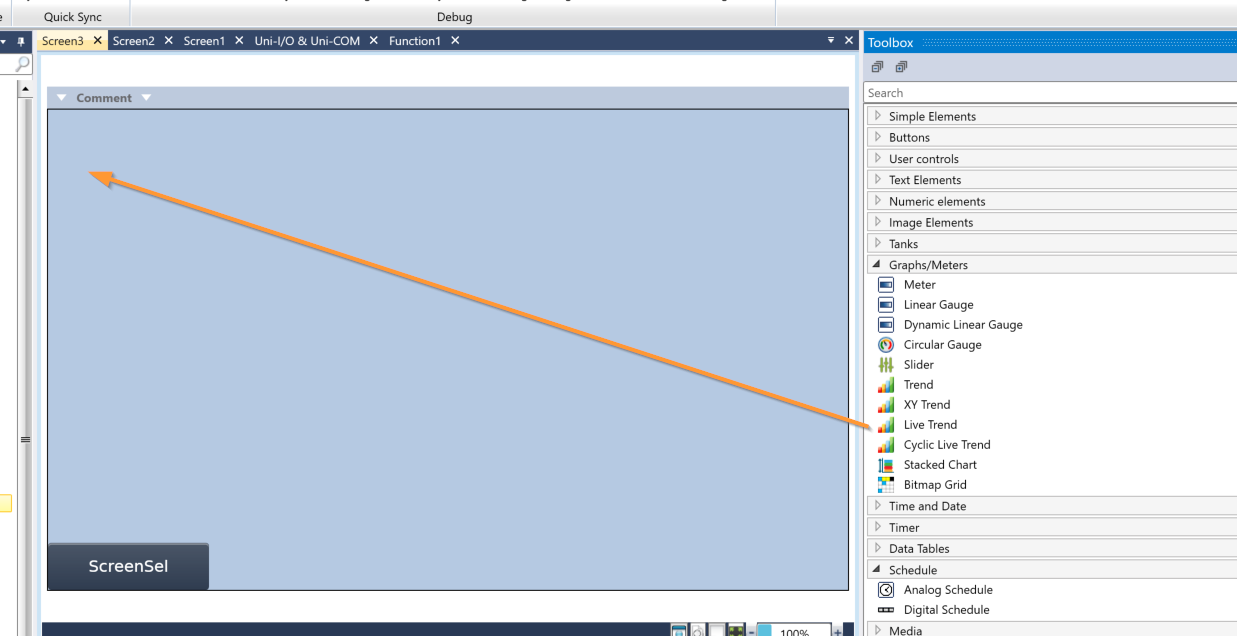
The Cyclic Live Trend component has been added.
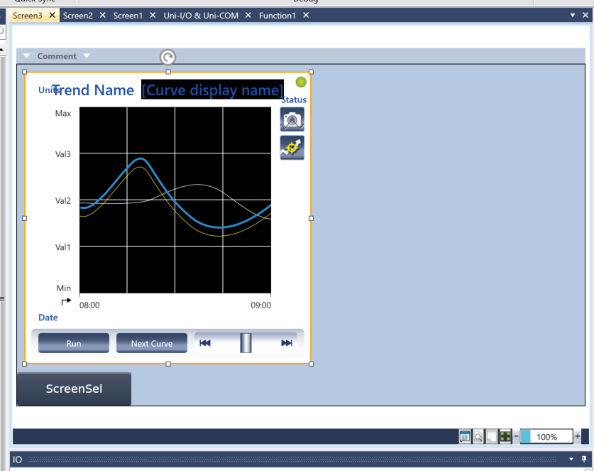
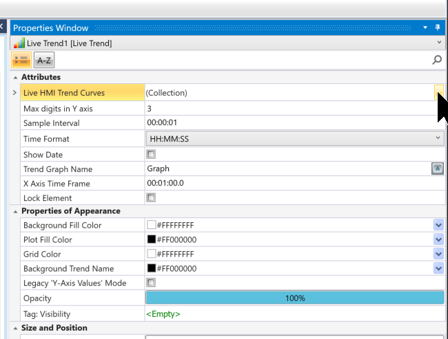
To set the variables to be displayed in the Trend, click Attributes → Live HMI Trend Curves.
This is the Curve addition screen.
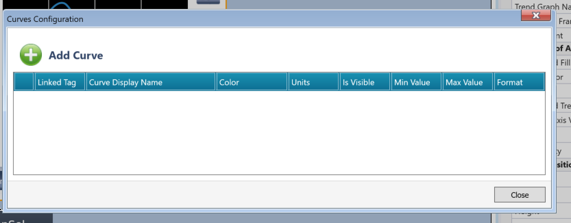
Click Add Curve, link the Linked Tag to a PLC Runtime Tag, and change each Curve’s color in the Color column.
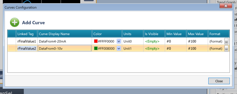
Done!
You can check the operation from this video.